Physical Not Included: How SSMs Reformulate Klei’s Magic into Scalable Science
Deconstructing Oxygen Not Included’s thermal magic to explore GPU-native parallel physics, State-Space Models (SSMs), and Mamba’s Physical AI potential.
Game Engine
AI
Physics
Research
Author
KaguraNaku
Published
March 24, 2026
Introduction
I’ve been wanting to write this blog for so long. Although I have been tormented to the brink of death by this hardcore masterpiece—wrestling with Liquid Locks, complex Pipeline Cycles, and thermal management—I still love it. To me, it is one of the greatest independent games ever made, a perfect playground of chaos and logic.
Paradigm Shift: From Sequential Simulation to Predictive State-Space Models
The Curse of Temporal Coupling
We have long relied on FEA-inspired1 methods to simulate complex physics in games. This is not just limited to Oxygen Not Included, but spans the entire genre of simulation-heavy titles like Workers & Resources: Soviet Republic (which I prefer even over ONI), the Anno series, and Tropico. These titles all share a common “curse”: the more realism we pursue, the harder it becomes for the CPU to keep up with the overwhelming grid-based workloads. We’ve been forced to lean on the sheer size of L3 caches to mask the underlying memory latency, but obviously, not every player has a 9800X3D. Yet we are still just brute-forcing a sequential bottleneck.
The mathematical model of grid-based methods can be simplified as shown in Equation 1: \[
\mathbf{u}_{t+1} = \mathcal{F}(\mathbf{u}_t, \Delta t)
\tag{1}\]
As we can see, the next state \(\mathbf{u}_{t+1}\) is tightly coupled to the current state \(\mathbf{u}_t\) and the time step \(\Delta t\). This creates a strict serial dependency, meaning the CPU spends most of its cycles stalled, waiting for memory synchronization or cache coherency.
Parallel against Serial
A Hypothesis: Logical Parallelism
At this point, I’d like to propose a hypothesis: Why not “predict” instead of “simulate”? Why not pursue “logical parallelism” over simple “physical parallelism”?
The current state is not an isolated point, but a temporal propagation of its predecessors. If we can decouple these temporal dependencies using SSMs (State Space Models), grid-based tasks become naturally GPU-native. We are no longer limited to solving thousands of grids for a single time step; instead, we can leverage the GPU’s dense compute units to resolve thousands of future states across the timeline in one fell swoop.
Have you played games by Paradox, such as the Hearts of Iron (HOI) series? To me, they are the ultimate counter-examples. Their simulation of global logistics and division movements is a nightmare of sequential coupling—the exact architectural bottleneck we are finally equipped to break.
Redefining DLSS: Deep Learning Super Speed
At the architectural level, traditional engines treat the simulation grid as a linearized 1D array. To maintain logical consistency, they are forced into a strict sequential iteration—updating states cell-by-cell, tick-by-tick. While this ensures precision, it remains tethered to the clock speed of a single thread, struggling to escape the von Neumann bottleneck.
My core insight is to bridge this gap using a fundamental concept from Computer Vision. If we strip away the color channels, a simulation grid is mathematically isomorphic to a 2D tensor (e.g., a 224x224 grayscale image).
The conceptual bridge is rooted in the mathematical duality of their filtering operations (Equation 2 and Equation 3):
CNN (Spatial Perception): \[Y = X * K_{\text{spatial}}, \quad K_{\text{spatial}} \in \mathbb{R}^{h \times w} \tag{2}\] Where \(K\) is a kernel that perceives spatial patterns across the grid to resolve feature maps.
\(\bar{K}\) is the kernel that projects the system’s DNA across the timeline to resolve the future;
\(\mathbf{\bar{B}}\) is the input matrix, which projects the current input into a hidden state;
\(\mathbf{\bar{A}}\) is the state transition matrix. Raising it to the power of \(k\) (\(\mathbf{\bar{A}}^k\)) is the mathematical magic that allows us to “fast-forward” the system’s internal state \(k\) steps into the future without iterating through \(1, 2, \dots, k-1\);
\(\mathbf{C}\) is the output matrix, which projects this hidden state back into our observable output.
SSM Conv. form works on time series
NoteDerivation: From Sequential Physics to Parallel Convolution (Click to expand)
How does an SSM actually turn sequential physics into a parallel convolution? Let’s walk through the transformation step by step. We start with the discrete-time state space model (the bread and butter of control theory):
Here \(h_t\) is the hidden state (e.g., temperature distribution), \(x_t\) is the input (e.g., heater power), and \(\mathbf{\bar{A}}, \mathbf{\bar{B}}, \mathbf{C}\) are constant matrices derived from the continuous physics. This recurrence is strictly sequential: to compute \(h_t\) you need \(h_{t-1}\).
The matrix is a Toeplitz matrix—each row is a shifted copy of the kernel. Multiplying this matrix with the input vector computes all outputs in one go, without iterating over time steps. This is exactly the parallel-friendly operation that GPUs excel at, just like a 2D convolution in a CNN.
So, by absorbing the recurrence into a precomputed kernel, we replace the serial loop over time with a single, highly parallel matrix operation. That’s the essence of turning Klei’s sequential “magic” into scalable science.
In CV, a CNN uses its receptive field to perceive spatial patterns across an entire image in a single GPU pass. By leveraging the convolutional duality of SSMs, we can apply this same logic to time. We treat the future timeline as an additional dimension of the state tensor, effectively creating a spacetime receptive field.
Instead of waiting for \(t\) to finish, we “snap” the entire temporal window into existence as a unified compute task. Causal convolutions act as the mathematical guarantee, ensuring that even in this parallel surge of computation, the information flow respects temporal entropy.
What makes this mapping worth noting is how it aligns with the engine’s actual memory layout: the flattened 1D world state becomes the sequence dimension for the SSM, turning the double loop over space and time into a single parallel scan.
In systems programming, when the physical layout matches the logical abstraction, it usually pays off in predictable performance. This is simply one of those cases.
Redefining RTX: Real-Time Temporal eXecution
That being said… does anyone even remember we just wanted to make Klei’s “magic” a bit more realistic at first? Maybe I’ve spent so much time on “DLSS” that things are getting a bit “Oxygen Not Included”, but the real point of using SSMs for Real-Time Temporal eXecution was always about restoring physical continuity from the game’s approximations.
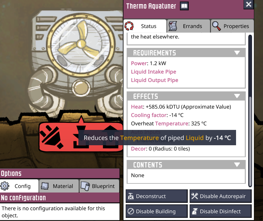
This is a real problem I encountered: the Thermo Aquatuner (TA) in ONI. No matter what coolant is used, and regardless of the input temperature, the TA magically subtracts a constant \(14^\circ\text{C}\) from the flow—a discrete, rule-based leap that ignores the complexity of real-world thermal exchange. I’ve come to call this “Klei’s Magic”.
Pipeline Liquid Cooling
This has created an interesting phenomenon: when calculating heat transfer, the system appears almost “scientific” because it respects the Specific Heat Capacity (SHC) of the liquid (Equation 7).
\[Q = m \cdot C_p \cdot \Delta T \tag{7}\]
where:
\(Q\) is the thermal energy moved, measured in DTU/tick;
\(m\) is the liquid mass (\(10\text{ kg}\));
\(C_p\) is the Specific Heat Capacity (in \(\text{DTU/kg}\cdot^\circ\text{C}\));
\(\Delta T\) is the constant \(14^\circ\text{C}\) offset.
However, as we can see, this pseudo-fidelity comes at a peculiar cost: simplifying the entire thermal evolution into a single, hard-coded constant \(\Delta T = 14^\circ\text{C}\).
The piecewise function above (Equation 8) illustrates the compromises Klei made when simulating thermal dynamics.
Assuming a naturally running, self-consistent system—and ignoring sudden chaotic inputs like player interventions—a Linear Time-Invariant (LTI) SSM can model this state machine with true mathematical continuity, gracefully replacing the brute-force subtraction of a hard-coded constant.
Instead of a discrete \(14^\circ\text{C}\) jump, we return to the fundamental continuous-time differential equation for heat exchange (akin to Newton’s Law of Cooling), expressed in the standard continuous State-Space form (Equation 9 and Equation 10):
\(h(t)\) is the continuous internal temperature state of the liquid;
\(\mathbf{A}\) is the continuous thermal decay matrix (derived from thermal conductivity and SHC), governing how the temperature naturally evolves over time;
\(x(t)\) represents the external continuous heat extraction driven by the Aquatuner;
\(\mathbf{B}\) determines how this heat extraction influences the liquid’s temperature state;
\(y(t)\) is the final observable output temperature \(T_{out}\).
Through discretization techniques like Zero-Order Hold (ZOH), this continuous ODE is mathematically transformed into the discrete matrices (\(\mathbf{\bar{A}}, \mathbf{\bar{B}}\)) we saw in Equation 3 of the “DLSS” section. This mathematical transformation is exactly what allows the GPU to compute the continuous cooling curve as a parallelized temporal convolution, restoring the beauty of physics without the serial CPU bottleneck.
Code
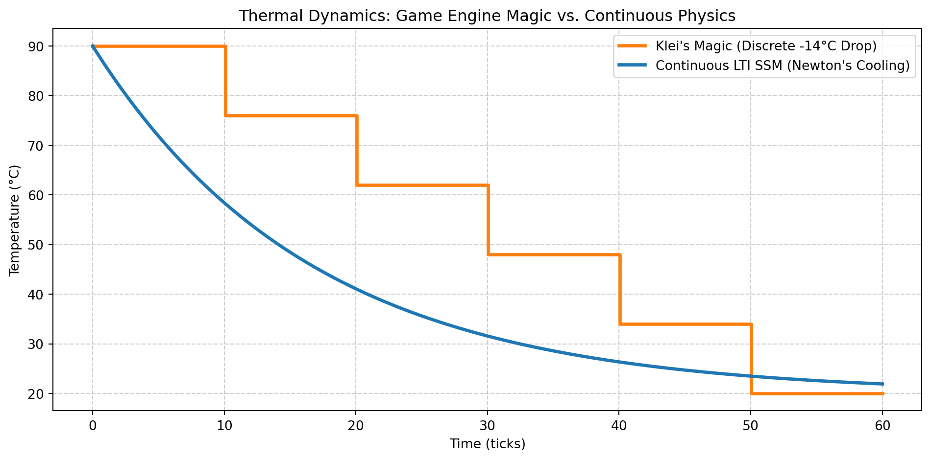
import numpy as npimport matplotlib.pyplot as plt# Time array (0 to 60 ticks)t = np.linspace(0, 60, 500)# 1. Klei's Magic: 14-degree drop every 10 ticks (Hard-coded step function)def klei_magic(t): drops = np.floor(t /10) temp =90- drops *14return np.maximum(temp, 20) # Cap at an arbitrary ambient 20°Ctemp_klei = klei_magic(t)# 2. Continuous LTI SSM (Newton's Cooling: h_dot = A*h)T_env =20T_0 =90k =0.06# Thermal decay constant (matrix A equivalent)temp_ssm = T_env + (T_0 - T_env) * np.exp(-k * t)# Plottingplt.figure(figsize=(10, 5))plt.plot(t, temp_klei, label="Klei's Magic (Discrete -14°C Drop)", color="#ff7f0e", drawstyle="steps-post", linewidth=2.5)plt.plot(t, temp_ssm, label="Continuous LTI SSM (Newton's Cooling)", color="#1f77b4", linewidth=2.5)plt.title("Thermal Dynamics: Game Engine Magic vs. Continuous Physics")plt.xlabel("Time (ticks)")plt.ylabel("Temperature (°C)")plt.grid(True, linestyle="--", alpha=0.6)plt.legend()plt.tight_layout()plt.show()
Figure 1: Visualizing the paradigm shift: The rigid steps of Klei’s Magic vs. the smooth, differentiable trajectory of a continuous LTI SSM.
The Modernization Refit: Injecting Chaos with Mamba
Our LTI SSM provides a mathematically rigorous foundation. Much like a classic dreadnought relies on pre-calculated trajectories to efficiently project power over vast distances, our global convolution predicts thousands of future ticks in a single computational pass. However, this architecture harbors a fundamental flaw: it assumes a completely predictable target. In technical terms, a strict LTI system inherently struggles to adapt to sudden, non-linear state transitions.
Remember my earlier caveat: “ignoring sudden chaotic inputs like player interventions”? In Oxygen Not Included, chaos is the only constant. What if a Duplicant suddenly pulls the automation wire, cutting power to our Aquatuner at \(t=50\)? What if the liquid temperature drops below \(0^\circ\text{C}\) and undergoes a phase change into ice, instantly altering the thermal decay matrix \(\mathbf{A}\)?
Standard SSMs are constrained by their Linear Time-Invariant (LTI) nature. The matrices \(\mathbf{\bar{A}}\) and \(\mathbf{\bar{B}}\) are rigidly static. Once the temporal convolution kernel \(\bar{K}\) is compiled, the laws of physics are locked in. It simply cannot handle non-linear edge cases or the inherently unpredictable nature of player interactions.
To make our dreadnought survive modern chaotic warfare, it needs a modernization refit. We must introduce Mamba.
Mamba upgrades the classic SSM by introducing Selective State Spaces. To understand how it works, let’s look at the mathematical “diff” between the discrete recurrent update of a standard LTI SSM and Mamba’s selective variant:
where the matrices are no longer rigidly static, but are generated on the fly at each tick \(t\) based on the current input \(x_t\):
\(x_t\) is the real-time contextual input (e.g., the current automation grid status or ambient temperature);
\(\mathbf{\bar{B}}_t = \mathbf{\bar{B}}(x_t)\) and \(\mathbf{C}_t = \mathbf{C}(x_t)\) are data-dependent matrices. They selectively filter how much of the current game input enters the physical state, and how much of that state is projected to the output;
\(\Delta(x_t)\) is a data-dependent step size that fundamentally alters the state transition matrix (\(\mathbf{\bar{A}}_t = f(\mathbf{A}, \Delta(x_t))\)) in real time.
This mechanism grants the system dynamic context-awareness. If the player cuts the power, \(\mathbf{\bar{B}}_t\) can instantly drop to zero, blocking heat extraction. If the water drops below \(0^\circ\text{C}\), the step size \(\Delta(x_t)\) modifies \(\mathbf{\bar{A}}_t\) to reflect the phase change into ice. Mamba effectively acts as a continuous, differentiable if-else router, gracefully handling non-linear boundary conditions without resorting to crude game-engine branching.
But here lies the ultimate technical dilemma: if our matrices change at every tick based on player inputs, we can no longer precompute the causal convolution kernel \(\bar{K}_k = \mathbf{C}\mathbf{\bar{A}}^k\mathbf{\bar{B}}\). Does this mean we fall back to the sequential CPU loop, ruining our “Logical Parallelism”?
Not at all. To preserve the firepower of the dreadnought, Mamba swaps out the causal convolution for a hardware-aware algorithm known as the Parallel Associative Scan.
If we unroll the selective recurrence from Equation 12 (assuming \(h_0 = 0\)), the state at time \(t\) expands to:
The cumulative product \(\prod_{i=j+1}^{t} \mathbf{\bar{A}}_i\) represents the dynamically changing physical laws accumulating over time. It directly replaces the static matrix power \(\mathbf{\bar{A}}^{t-j}\) from our classic LTI model;
Because \(\mathbf{\bar{A}}_i\) changes at every tick, this massive sequence cannot be pre-computed into a simple convolutional kernel \(\bar{K}\);
However, because matrix multiplication is associative (i.e., \((\mathbf{A}_1\mathbf{A}_2)\mathbf{A}_3 = \mathbf{A}_1(\mathbf{A}_2\mathbf{A}_3)\)), the GPU does not have to compute this chain strictly chronologically from past to future.
Even though the state transitions are dynamic and seemingly sequential, Mamba treats them as these associative blocks (conceptually similar to a parallel prefix sum). By leveraging the GPU’s SRAM hierarchy, it computes these dynamic sequences in highly optimized parallel chunks. Thus, Mamba achieves the holy grail: it retains the blazing-fast, non-blocking parallel execution of our “DLSS” architecture, while fully embracing the unpredictable, non-linear chaos of a living game world.
Conclusion
We have evolved from deconstructing an initially unscientific “Klei magic” to exploring the bleeding-edge possibilities of GPU-native parallel physics. Much like the invention of the microwave oven—where a melted candy bar in a radar lab sparked a revolution—our frustration with a hard-coded \(14^\circ\text{C}\) temperature drop gave birth to a rather intriguing inquiry into State-Space Models and Mamba.
Ultimately, I hope this exploration is seen as more than just an over-engineered fix for a game mechanic. Perhaps it can serve as a small glimpse into the future of simulation. By bridging classical thermodynamics with modern AI architectures, I hope we are inching closer to the era of Physical AI—where chaos and logic might finally run in true parallel.